Intuition: Comparing Hypotheses with Data

 

In the last section, we discussed the underlying logic of hypothesis testing. Let us now turn to a more concrete example of conducting hypothesis test on a specific type of parameter: population proportions. Recall in the previous chapter, we also started with the question of estimating proportions. So we will follow the same order, first looking at testing claims about proportions, then testing claims about means. This may be a bit different from the textbook, but you can choose to follow either order.

From the class data, I have found something that sets the hybrid Math 15 classes from the same traditional sections that I taught in the past: there seem to be more women in hybrid sections than men. In the class data, we see that there are 45 responses from women, and 29 responses from men. Using the symbols introduced earlier, we will represent our qualitative data as follows:

 

 

Does this mean that hybrid sections are for some reason more "popular" among female students? If the answer is yes, then it will be very valuable for the college to have this information, since it may help us schedule hybrid sections in the future (for example, on Fridays when parking is more readily available).

However, we want to be sure that the alleged gender disparity is not just a fluke: if we toss a fair coin 74 times, then it is certainly possible to get 45 heads, although such an outcome is quite unlikely, because you would expect close to half of the tosses turn up heads. So we'd better have a way to say that 45 (sample proportion of 60.8%) is a little too far from 37 (50%) for this to occur by chance, but we will need also be clear what we mean by "occur by chance." When this unlikely event does happen in the 50/50 split scenario, and we mistakenly concluded that more than 50% students are women, a Type I error occurs. Based on our discussion in the last section, we want to control this type of error by choosing a small . How small? Just like in confidence interval, where a variety of confidence levels are in use, we can choose  to be as small as we like. For now, let's use the common value of .

Intuitively, we reasoned that "more than half of the hybrid Math 15 students are female", because "60.8% (the sample proportion) is too high above the 50%." Let us make this argument more official by using hypothesis testing.

As we emphasized last time, the most important step in hypothesis testing is setting up the null and alternative hypothesis. In our case, because our suspicion is that there are more women, so if you use  for the proportion of women, this leads to a right-tailed test (“>”  

 

 

In plain English, , always containing the equal sign, says exactly half are women, and  is our original claim: more than half are women.

Test Statistic

 

The second step in hypothesis testing is to convert our data and null hypothesis into a single numerical summary, also called the test statistic. Intuitively, the test statistic measures how "far away" our sample proportion is from the alleged 50% population proportion according to . The calculation of test statistic is familiar from the chapter on confidence interval of proportions:

 

 

The various symbols appearing in the test statistic formula are as follows:

1.       The sample proportion of female studnets:  

2.       The population proportion of female students according to the null hypothesis: p = 0.50

3.       The population proportion of male students according to the null hypothesis: q = 0.50

4.       The sample size: n = 45 + 29 = 74

Similar to our discussion in testing a claim about means, this test statistic is also based on Central Limit Theorem for Sample Proportions:

1.        The sampling distribution for the sample proportion  is approximately normal

2.       The mean of  is equal to , i.e.  

3.       The standard deviation of   is equal to , i.e.  

If we recognized that p and  are the mean and standard deviation of the sample proportion , then the test statistic formula is another way to convert a non-standard normal distribution to the standard normal, hence the letter “Z”.

Notice in confidence interval (see the previous notes), we used this test statistic to construct the margin of error (we also discussed it as finding the cut-off values from the area in the middle, i.e. confidence level). The main difference is that in Confidence Intervals, we are using  to predict a range for ; while in Hypothesis Testing, we are comparing  with p to see whether the two are significantly different. The way we interpret the test statistic is exactly the same as how we look at the Z-scores: if the test statistic is more than 2 standard deviations away from zero, then it has gone "too far".

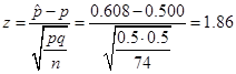
In our scenario, the test statistic comes out to be:

 

 

This is somewhat marginal according to the criteria of 2 standard deviations. So to decide whether this could "occur by chance", we need to do one of two things that help us arrive at the final decision.

Making Decision with P-value

 

Option 1 is called the "P-value" method (be careful of the multiple "P" used in different contexts), which is the default method used in the book. It is named because we need to put a probability on how likely it is to see data like ours, when  is true. Because the Z (standard normal) distribution is continuous, to find the probability, you must look at an area. 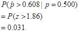So the natural thing to do to characterize "data like ours" is to look at the area to the right of our test statistic, since any test statistic landing in this tails will support our claim (larger than 0.50). Using the normal calculator in GeoGebra, we found that:

 

As we mentioned in the introduction to hypothesis testing, this probability gives us an idea of how the evidence measures against :

·         Interpretation of p-value: "If 50% of the students are female, then there is a 3.1% chance that in a sample of 74 students, 45 or more of them are female."

Alternatively, you can also refer to the sample proportion in your P-value interpretation:

• I"If 50% of the students are female, then there is a 3.1% chance that in a sample of 74 students, 60.8% or more of them are female."

 

I know this is a rather long sentence, but trust me, every word in the definition of P-value is necessary to convey the full meaning -- it's a rather complex idea that cannot be expressed with fewer words. If you have trouble reading the above sentence, I would suggest that you take a pause, and read the sentence out loud to yourself.

Here is the graph that illustrates the different views of the P-value:

Comparing the P-value to our significance level , we basically concluded that getting a sample proportion of 60.8% or more is very unlikely to occur by chance. So following the logic of hypothesis testing, we will decide to reject , i.e. supporting our original suspicion that more than half of the students are female (remember the double-negatives?). In statistical language, we often state that "there is significant evidence to support that the majority of students in hybrid Math 15 are female," and we are done!

Let's pause for a second and take a look at why the fuss about null/alternative hypothesis is necessary. In order to calculate the p-value, we must have some type of ground truth so that we can use to calculate the probability of our evidence. , the null hypothesis, provides a ground truth. In fact, p-value can be roughly stated as the following statement:

·         General Interpretation of p-value: "the chance of seeing the evidence more extreme than the data, given that  is true."

Although our interest is always on, we arrive at our conclusion by negating its opposite , and p-value is a way for us to point to the data and say "that's ridiculous."

P-value is the preferred method in most applications of hypothesis testing because of the simplicity in decision rule: if P-value < , you have a significant result (either <, >, or , depending on ). However, historically, it was invented after the more traditional method of using critical values to arrive at the same decision.

Binomial Test: An Alternative to Using the Z Test Statistic

A final note on the p-value method: using the definition of p-value as a conditional probability ("the probability of getting data more extreme than yours, given that the null is true"), there may be multiple methods of computing the p-value. In fact, the method of converting the proportion data to standard normal was used because of limited computational resources, since computing the binomial probabilities with  is a bit tricky in the old days of sliding rules. By using the Binomial calculator that we introduced in the chapter on discrete probability distributions, we can also use a binomial distribution with , and  to evaluate the p-value: 

When the sample size  is fairly large, the p-value obtained from using the standard normal  serves as a fairly good approximation of the p-value obtained from the binomial distribution, and you can use either method in testing one proportion. If a binomial distribution is used to calculate p-value, then the hypothesis test is also called “binomial test” (as opposed to “Z-test for a proportion”), if it is included in different statistics software.

Making Decision with Critical Values (optional)

 

Option 2: instead of comparing p-value with  (both are areas under the Z curve), we could also directly compare the test statistic with the critical value(s), since they are both Z-scores. In our earlier example, since  is right-tailed, we will be looking for the critical value (C.V.) that marks the 0.05 area to the right of the Z-score. In other words, we are looking for:

Using our normal calculator to solve for Z-score again, we obtain C.V. = 1.64. We call the area to the right of critical value "critical region". When you look at where the Z-test statistic stands, it is certainly inside the critical region. So we have arrived at the same decision as Option 1: we will reject , the proportion of female students is indeed over 50%.

Comparing the p-value method with the traditional method, you can see that they are two different ways to make the same decision with regard to : the p-value method uses area for comparison, and the traditional method uses the Z-scores. Although one-tailed tests are relatively straightforward, the two-tailed tests can be a little tricky: the p-value should include the area in BOTH the left and right tail, and the traditional method will rely on TWO critical values, one associated with a critical region in each tail.

Hypothesis Testing and Proof by Contradiction

 

So in a nutshell, here is how we confirmed our initial suspicion that more women than men are taking the hybrid Math 15:

1. Assume  according to .

2. Compare our sample proportion  with 0.50 and summarize the comparison with the test statistic.

3. Use either the p-value (compared with ) or the test statistic (compared with critical value) to conclude that  is simply too far from 0.50 to occur by chance.

4. Revisit the assumption in Step 1:  must be false, hence we have proved our point that .

If you have taken a philosophy course that deals with logic, you may have recognized that this type of argument is also known as "proof by contradiction". To give a simple example, imagine that if you want to show I am not a vegetarian, after I have told you that I like steaks. So your reasoning goes something like the following:

1. Assume Dr. Lin is vegetarian.

2. Vegetarians don't eat steaks.

3. But Dr. Lin likes steaks.

4. So there is a contradiction. The assumption that he is vegetarian must be false.

Of course, hypothesis testing does not deal with black-and-white situations like this. The real-world scenarios have many shades of gray. Suppose you are trying to test the same claim "Dr. Lin is not a vegetarian", and I told you that I like sushi. Is there a contradiction if you assume I am vegetarian? Well, apparently there are many sushi restaurants in California that serve vegetarian sushi, so the probability that a vegetarian likes sushi, although fairly small, is certainly not zero! (a probability of zero will be equivalent to a contradiction). Should you reject the null hypothesis that I am vegetarian? This will depend on a number of things: first, you will need some type of mathematical model that predicts the probability of a vegetarian liking sushi, which gives us the p-value; then you will need to compare the p-value with a pre-determined significance level. If the p-value is smaller than $\alpha$, then this means that it must be a miracle that you just met a sushi-loving vegetarian, so you have effectively found a contradiction and proved that I am not vegetarian. On the other hand, if the p-value turns out be quite large, then you will "fail to reject null hypothesis." In simple terms, you just don't have enough evidence to prove I am not vegetarian, which is quite different from proving I AM vegetarian! (remember the "guilty" and "not guilty"?)

Equivalent Statements in Stating the Conclusion

 

So here are the two conclusions again:

Fail to reject H0  not enough evidence to support Ha  p-value is large  test statistic is close to zero (outside the critical region)  if H0 were true, the data still could occur by chance

Reject H0  enough evidence to support Ha  p-value is small  test statistic is far away from zero (in the critical region)  if H0 were true, the data is not likely to occur by chance

It's useful to become familiar with all the equivalent statements so that you can see hypothesis testing from all the angles. Perhaps the most important piece is the understanding of p-value, which we will revisit when we look at the hypothesis testing of means.

Summary: Hypothesis Test about One Proportion

 

First let’s summarize the example above in terms of the five components of a hypothesis test. To test the claim that more than half of the Math 15 students are female, we proceed as follows:

a)      State the null and alternative hypotheses.
                  

b)      Show the test statistic.
 

c)       Show the P-value

d)      State the decision of your hypothesis test
Reject the null hypothesis (since P-value < α)

e)      State your conclusions in words a non-statistician would understand.
There is significance evidence to show that more than 50% of the students taking Math 15 are female.