Review of Hypothesis Testing

 

We've spent a lot of time on hypothesis testing, one of the two main paradigms of statistical inference.  To briefly summarize, each hypothesis test consists of the following components:

1. 
   
    and  
   
2. Test statistic
3. P-value and its meaning
4. Decision
5. Interpretation of the results.

For example, if we are testing a claim about the population mean (e.g. the average height of male students in stats class is more than 68 inches) without any information about the population standard deviation , the appropriate test statistic will be the Student's t, and the P-value will be right-tailed. If the P-value is very small (less than the significance level), it means that the null hypothesis, if it were true, has led to some unlikely results. Thus  should be rejected, leading to a significant result.

This whole paradigm, although it can feel unnatural at first, is actually the standard framework for statistical decision making for all hypothesis tests, and the meaning of P-value is quite universal: it measures the strength of the evidence against . 

Comparing Two Populations

 

However, to see how to apply hypothesis test to real-life scenarios such as your term project, we are often faced with insufficient information regarding what we should be comparing our parameter to. What if we don't know the nation average of male students in this age group? Much more common is the scenario in which we are comparing two populations, and our primary interest is how their main parameters (either the mean or proportion) compare with each other. For example, you may be wondering: do women spend more time getting ready in the morning? Does a supermarket offer cheaper prices than its competitors? (These are actually real questions from past Math 15 student projects)

At first, this seems to present a rather insurmountable problem: how are we supposed to compare two means, if we don't have any clue about the likely value of either one of them? It turns out that this is not such a big deal after all, because the following nice property of the normal distribution:

·         If , and , then their difference is also Normal: .

This turns out to be a life saver for the problem of comparing two means: since the difference of two sample means is supposed to be normal, in hypothesis testing, we just need to compare it with , the difference between the population means in order to see how likely this is to occur (hence the P-value). With calculus, we can also show that the difference sample means can also be described by a different form of Central Limit Theorem:

 

Ideally, to conduct such a test, we would like to have both  and . But the reality is such that the two standard deviations are almost never available. This situation is not new -- in the previous module, we saw that we can still use the t statistic to test the mean without , i.e.

 

Now we just need to make a similar adjustment for the difference of two means, since it still follows a normal distribution. The t statistic for the two-sample test is given by:

 

At first it seems rather intimidating. But here is the most common scenario for comparing two means: often we are simply interested in whether one mean is greater than, less than, or not equal to the other, so the difference  in all of the examples we will be showing.

Example: Comparing Height of Male v.s. Female Students

 

Let's start with an example with a rather obvious conclusion: on average, are male students taller than female students? Intuitively, we know the answer is "yes", but it's helpful to examine the actual distributions shown in the class data by looking at the box plots:

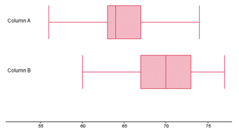
The top and bottom graphs correspond to the data from female and male students, respectively.

Although we can't see the means from the boxplot, we can estimate where they are. It appears that relative to the variation in each sample, the difference in mean is significant. But to be sure, we will need to conduct a hypothesis test. We will start with the hypotheses. Using subscript f to represent female, m to represent male, our hypotheses are:

It's useful to note the alternative forms of these hypotheses, which makes it clear that it's a type of right-tailed test:

  (also written as )

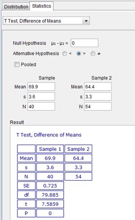
Using GeoGebra, we can also obtain the sample statistics as follows:

Male	Female

 

Evaluating the t statistic using these values, we found:

Notice that we have replaced  with 0 according to the null hypothesis (this may change if we have specific values in the claim, i.e. "on average, men are at least 3 inches taller than women").

The last piece of the puzzle before we find the P-value is the degree of freedom, which has a fairly complex form that you can locate in the textbook. Since it's typically not an integer, it's common for people to use the smaller of the two sample size less one to approximate this degree of freedom (39 in our case). If you are interested in the exact degree of freedom, the TI-calculator or software like GeoGebra can also compute this value.  (you will need to go to the Statistics calculator, “T Test, Difference of Means”. See the screen capture below)

By using the probability  (using either your calculator for GeoGebra), we have arrived at the P-value of this test: P-value is almost zero, since the test statistic is rather far away from the mean.

Just like the hypothesis testing  for one mean, the P-value  for this test can also be interpreted in the same framework of “the chance of seeing the evidenced, given that H0 is true”, except that the sampling distribution is the difference of the two sample means:

·         Interpretation of P-value: if the population means for male and female are the same, then the chance of getting a difference in sample means of more than 5.5 inches (69.9-64.4=5.5) is practically 0.

The following graph illustrates the relationship between this interpretation of the P-value, the sampling distribution, and the test statistic (the scale is exaggerated a bit to show the P-value):

 

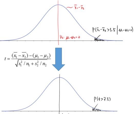
So what does this mean? A tiny P-value indicates a very significant result: the difference in sample means is 5.5 inches, which is much larger than 0, even considering that the standard deviations were 3.6 and 3.3, respectively. In fact, you can imagine the men within one standard deviation of the mean are almost invariably taller than the women within 1 standard deviation of their mean. This confirms our impression from comparing the two boxplots.